
Best ARIMA Model Training Tools to Buy in July 2026
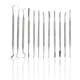
CYNAMED Stainless Steel Spatula Wax & Clay Sculpting Tool Carver Set (12PK)
- VERSATILE DOUBLE-SIDED TOOL FOR DIVERSE SHAPES AND APPLICATIONS.
- IDEAL FOR CARVING, CUTTING, SCRAPING, AND MORE-LIMITLESS CREATIVITY!
- DURABLE STAINLESS STEEL DESIGN ENSURES LONG-LASTING PERFORMANCE.


Clay Sculpting Tools, Double-Ended Clay Sculpting Tool Stainless Steel Modeling Clays Tools Implement for Modeling Embossing Sculptings and Shaping Miniature
-
VERSATILE DOUBLE-HEADED TOOLS EASILY HANDLE DIVERSE SCULPTING TASKS.
-
DURABLE STAINLESS STEEL CONSTRUCTION ENSURES LONG-LASTING, RUST-FREE USE.
-
COMPACT DESIGN SAVES SPACE WHILE DELIVERING EFFICIENT CARVING PERFORMANCE.
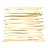
Honbay 10-Piece Double Ended Wooden Mini Modeling Tools Clay Sculpture Tools for Cutting, Carving and Smoothing
- 10 VERSATILE TOOLS FOR CUTTING, CARVING, AND SHAPING CLAY.
- ERGONOMIC WOODEN DESIGN ENSURES COMFORT AND CONTROL WHILE CRAFTING.
- IDEAL FOR ALL SKILL LEVELS-PERFECT FOR BEGINNERS AND PROS ALIKE!

Keadic 87Pcs Gundam Model Tool Kit Hobby Building Tools Kit Tools Gunpla Tool Kits Modeler Basic Tools Craft Set Professional Gundam Model Tools Kit for Hobby Building
- COMPLETE ALL-IN-ONE KIT FOR EVERY MODELING PROJECT YOU CAN IMAGINE!
- PRECISION TOOLS PERFECT FOR BEGINNERS AND SEASONED MODEL MAKERS ALIKE.
- LIGHTWEIGHT, PORTABLE STORAGE FOR CRAFTING ANYTIME, ANYWHERE!

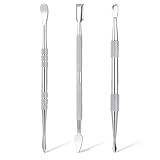
The Army Painter Clay Sculpting Tools - Set with Three Double Ended Stainless Steel Dab Tool, Polymer Clay Tools for Modeling Plastic, Resin, and Metal Miniatures - Green Stuff Putty Tool Clay
-
TOP 3 TOOLS FOR PRECISE MINIATURE MODELING & REPAIRING!
-
DURABLE STAINLESS STEEL: BUILT TO LAST FOR EVERY PROJECT!
-
PERFECT SIZE FOR WARGAMERS: DETAIL YOUR MINIS LIKE A PRO!
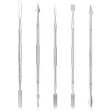
Clay Sculpting Tools, 5 PCS Stainless Steel Pottery Spatula Wax Carving Tools Set Double-Ended Polymer Clay Tools Kit for Modeling, Embossing, Sculpting and Shaping Miniatures
- VERSATILE DOUBLE-HEADED TOOLS FOR DETAILED CRAFTING AND MODELING.
- DURABLE STAINLESS STEEL CONSTRUCTION ENSURES LONGEVITY AND RESISTANCE.
- ERGONOMIC DESIGN REDUCES FATIGUE AND ENHANCES PRECISION DURING USE.

Waltool 15Pcs Gundam Modeling Tools Set, Basic Modeler Craft Hobby Tool for Gundam Models Assemble Building Repairing
- ALL-IN-ONE 15PCS KIT FOR ALL YOUR MODEL BUILDING NEEDS.
- DURABLE TOOLS DESIGNED FOR PRECISION AND COMFORT IN CRAFTING.
- PORTABLE STORAGE BOX FOR EASY ORGANIZATION ON THE GO.

YYaaloa 14pcs Set Plastic Crafts Clay Modeling Tool Pottery Carving Tools for Shaping and Sculpting for Ceramics Clay Pottery (Plastic Knife-14pcs)
- VERSATILE SET: 14 DURABLE TOOLS FOR ALL CLAY AND MODELING NEEDS.
- PRECISION DETAIL: PERFECT FOR CARVING, SHAPING, AND SMOOTHING TASKS.
- PORTABLE DESIGN: LIGHTWEIGHT TOOLS IDEAL FOR HOME OR SCHOOL USE.

DUGATO Clay Sculpting Tools (17pc Set) - Double-Sided Plastic Modeling Kit for Polymer Clay, Pottery, Fondant & Cake Decorating - Art & Craft Supplies for Beginners & Artists
-
17 ESSENTIAL TOOLS: COMPREHENSIVE SET TO UNLEASH YOUR CREATIVITY.
-
DURABLE & LIGHTWEIGHT: HIGH-QUALITY, EASY-TO-CLEAN TOOLS FOR LASTING USE.
-
VERSATILE PRECISION: DOUBLE-ENDED DESIGNS FOR INTRICATE DETAILS & TEXTURES.

Pottery Clay Sculpting Tools for Polymer, Yagugu 19Pcs Basic Wood Ceramics Carving Tool Supplies kit Accessories for Adults and Artists Modeling Shaping Building for Art&Craft
- VERSATILE 19-PIECE KIT: PERFECT FOR BEGINNERS AND EXPERTS ALIKE!
- HIGH-QUALITY DURABILITY: BUILT TO LAST WITH STEEL & HARDWOOD COMPONENTS.
- IDEAL GIFT CHOICE: PERFECT FOR ASPIRING ARTISTS AND POTTERY ENTHUSIASTS.
To train a model using ARIMA in Pandas, you first need to import the necessary libraries such as pandas, numpy, and statsmodels. Then, you can create a time series dataset and use the pandas.Series function to create a time series object.
Next, you can use the statsmodels.tsa.arima_model.ARIMA class to fit the ARIMA model to your time series data. This class takes three parameters: the endogenous variable (your time series data), the order of the ARIMA model (p, d, q), and an optional parameter for seasonal differences.
After fitting the ARIMA model, you can use the fit() function to train the model on your data. Finally, you can make predictions using the forecast() function and evaluate the performance of your model using metrics such as mean squared error or mean absolute error.
Overall, training a model using ARIMA in Pandas involves importing libraries, creating a time series dataset, fitting the ARIMA model, making predictions, and evaluating the model's performance.
How to tune the parameters of an ARIMA model in pandas?
In order to tune the parameters of an ARIMA model in pandas, you can follow the steps below:
- Install the pmdarima library if you haven't already, as it provides helpful tools for automatically selecting the hyperparameters of an ARIMA model.
pip install pmdarima
- Load your time series data into a pandas DataFrame and convert it to a Series.
import pandas as pd
Load the data
data = pd.read_csv('your_data.csv')
Convert to Series
ts = pd.Series(data['column_name'], index=pd.to_datetime(data['date_column']))
- Use the auto_arima function from pmdarima to automatically select the best hyperparameters for your ARIMA model.
from pmdarima import auto_arima
Fit the ARIMA model
arima_model = auto_arima(ts, seasonal=True, m=12, stepwise=True, trace=True)
- If you want to manually tune the hyperparameters, you can use the arima_order function from pmdarima to find the best parameters by grid search.
from pmdarima import arima_order
Find the best ARIMA parameters by grid search
order = arima_order(ts, max_order=5, seasonal=True, m=12) print("Best ARIMA parameters:", order)
- Once you have selected the best hyperparameters for your ARIMA model, you can fit the model and make predictions.
from statsmodels.tsa.arima_model import ARIMA
Fit the ARIMA model with selected parameters
arima_model = ARIMA(ts, order=(p, d, q)).fit()
Make predictions
predictions = arima_model.predict(start=start_date, end=end_date, dynamic=False)
By following these steps, you can successfully tune the parameters of an ARIMA model in pandas.
How to evaluate the performance of an ARIMA model in pandas?
To evaluate the performance of an ARIMA model in pandas, you can use the following steps:
- Fit the ARIMA model to your data using the ARIMA class from the statsmodels library. You can do this by specifying the order of the ARIMA model (p, d, q).
- Make predictions using the fitted ARIMA model on a test set of data.
- Calculate the Mean Squared Error (MSE) or another appropriate metric to evaluate the accuracy of the predictions.
- Plot the actual values against the predicted values to visually inspect how well the model is performing.
Here is an example code snippet demonstrating these steps:
import pandas as pd from statsmodels.tsa.arima.model import ARIMA from sklearn.metrics import mean_squared_error import matplotlib.pyplot as plt
Fit ARIMA model
model = ARIMA(data, order=(p, d, q)) model_fit = model.fit()
Make predictions
predictions = model_fit.predict(start=len(train), end=len(train)+len(test)-1, typ='levels')
Calculate MSE
mse = mean_squared_error(test, predictions)
Plot actual vs predicted values
plt.plot(test) plt.plot(predictions, color='red') plt.legend(['Actual', 'Predicted']) plt.show()
print(f"Mean Squared Error: {mse}")
Replace data, train, and test with your actual data and training/testing sets. Adjust the values of p, d, and q to optimize the ARIMA model. The lower the MSE value, the better the performance of the ARIMA model.
How to check for autocorrelation in time series data?
There are several methods to check for autocorrelation in time series data. Some of the common methods include:
- Autocorrelation Function (ACF): The ACF plots the correlation of a time series with itself at different time lags. A strong correlation at certain lags indicates autocorrelation. You can use statistical software like R or Python to calculate and plot the ACF.
- Partial Autocorrelation Function (PACF): The PACF measures the correlation between a time series and its lagged values after adjusting for the intermediate lags. A significant correlation at a certain lag indicates autocorrelation. Again, you can use statistical software to calculate and plot the PACF.
- Durbin-Watson Statistic: The Durbin-Watson statistic is a test for autocorrelation in the residuals of a regression model. If the value falls within a certain range (typically between 1.5 and 2.5), it suggests no autocorrelation.
- Ljung-Box Test: The Ljung-Box test is a statistical test to check for the presence of autocorrelation in a time series at different lags. You can perform this test using statistical software and check if the p-value is below a certain threshold (e.g., 0.05) to reject the null hypothesis of no autocorrelation.
By using these methods, you can determine whether there is autocorrelation in your time series data and make appropriate adjustments in your analysis.
How to create a lag plot in pandas for time series data?
To create a lag plot in pandas for time series data, you can use the shift() method to create lagged versions of your time series and then plot them against each other. Here's a step-by-step guide to creating a lag plot in pandas:
- Import the necessary libraries:
import pandas as pd import matplotlib.pyplot as plt
- Create a sample time series data:
data = {'date': pd.date_range(start='1/1/2021', periods=100), 'value': range(100)} df = pd.DataFrame(data)
- Create lagged versions of the time series:
df['lag1'] = df['value'].shift(1) df['lag2'] = df['value'].shift(2) df['lag3'] = df['value'].shift(3)
- Plot the lagged versions against each other:
plt.figure(figsize=(10, 6)) plt.scatter(df['value'], df['lag1'], color='blue', label='lag1') plt.scatter(df['value'], df['lag2'], color='green', label='lag2') plt.scatter(df['value'], df['lag3'], color='red', label='lag3') plt.xlabel('Value') plt.ylabel('Lagged Value') plt.legend() plt.title('Lag Plot') plt.show()
This will create a lag plot showing the relationship between the original time series values and their lagged versions. The x-axis represents the original values, and the y-axis represents the lagged values for different lag periods (1, 2, and 3 in this example).