
Best Graph Conversion Tools to Buy in July 2026
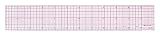
Westcott B-70 8ths Graph Beveled Ruler, 12 in
- PRECISION MEASURING WITH ZERO CENTERING FOR ACCURATE RESULTS
- DURABLE BEVELED EDGE PERFECT FOR CLASSROOMS AND EXTENSIVE USE
- TRANSPARENT DESIGN ENHANCES VISIBILITY FOR NEAT DRAFTING


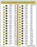
Fraction-Decimal Conversion Chart - 8 x 6 inches Decal, Inches to Millimeters. Toolbox Sticker, Engineer, Mechanic, in to mm Sticker Decal
- DURABLE VINYL: WEATHERPROOF AND LONG-LASTING FOR ANY SURFACE.
- SAFE & NON-TOXIC: PEACE OF MIND WITH EVERY USE.
- EASY APPLICATION: PERFECT FOR VEHICLES, LAPTOPS, AND MORE!

Spice Rack & Herb Organizer Set Magnet - Kitchen Cooking Guide Conversion Chart with Grilling Rubs & BBQ Seasoning Substitutions - Measuring Spoon Barbecue Accessories Gift Idea by Cave Tools
- MAXIMIZE FLAVOR WITH 20 ESSENTIAL SPICE PROFILES & PAIRINGS!
- PERFECT GIFT FOR BBQ LOVERS: EASY MEASURING & SEASONING MASTERY!
- MAGNETIZED FOR CONVENIENCE-COOK LIKE A PRO ANYWHERE YOU GO!
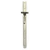
Big Horn 19206 6” STAINLESS STEEL POCKET RULER 1/64 1/32 Scales Decimal Conversion Chart Rulers
- ETCHED BLACK GRADUATIONS FOR CLEAR READING AND DURABILITY.
- DUAL-SIDED: 32NDS/64THS AND DECIMAL EQUIVALENTS FOR VERSATILITY.
- CONVENIENT SLIDING CLIP DOUBLES AS A DEPTH OR HEIGHT GAUGE.

SUNER POWER Waterproof 30W 12V Solar Battery Charger & Maintainer PRO, Built-in UltraSmart MPPT Charge Controller, 12 Volt Solar Panel Trickle Charging Kits for Car Automotive Boat Marine RV Trailer
-
MAXIMIZE ENERGY EFFICIENCY: UP TO 99% TRACKING, 98% CONVERSION.
-
BOOST BATTERY LIFE: ADVANCED 3-STAGE CHARGING FOR SAFE, EFFECTIVE RECHARGING.
-
WORRY-FREE OPERATION: AUTOMATIC CHARGING, FREE MAINTENANCE, AND FULL SAFETY.
To convert a SymPy expression into a graph, you can use the plot function provided by SymPy. First, you need to define the variables and the expression you want to plot. Then, use the plot function and pass in the expression along with the range of values you want to plot it over. SymPy will then generate a graph of the expression. Additionally, you can customize the appearance of the graph by specifying plot options such as the title, labels, colors, and line styles. This allows you to create visually appealing graphs of your SymPy expressions for better visualization and analysis.
What is the process for exporting a graph of a sympy expression to an image file?
To export a graph of a SymPy expression to an image file, you can use the matplotlib library, which is commonly used for plotting graphs in Python. Here is a step-by-step guide to export a graph of a SymPy expression to an image file:
- Install matplotlib library if you haven't already. You can install it using pip:
pip install matplotlib
- Create a SymPy expression using the sympy library. Here is an example expression:
import sympy as sp
x = sp.symbols('x') expression = x**2 + 2*x + 1
- Plot the graph of the expression using matplotlib. Here is an example code to plot the graph:
import matplotlib.pyplot as plt
x_vals = range(-10, 11) y = [expression.subs(x, val) for val in x_vals]
plt.plot(x_vals, y) plt.xlabel('x') plt.ylabel('y') plt.title('Graph of the expression: x^2 + 2x + 1') plt.grid(True) plt.savefig('graph.png')
- Save the image file using plt.savefig('filename') method. In this case, the image file will be saved as graph.png.
- You can find the image file in the same directory where your Python script is located. You can now view the graph in the image file.
- You can customize the graph further by changing the range of x_vals, the title, labeling, and other properties of the plot using matplotlib functions.
By following these steps, you can easily export a graph of a SymPy expression to an image file using Python.
How to adjust the size of the markers on a graph of a sympy expression?
To adjust the size of the markers on a graph of a sympy expression, you can use the marker_size parameter in the plot function. Here is an example:
import matplotlib.pyplot as plt import sympy as sp
x = sp.Symbol('x') expr = x**2
p = sp.plot(expr, show=False) p[0].line_color = 'b' p[0].marker = 'o' # Set marker style to circle p[0].marker_size = 10 # Set marker size to 10 p.show()
In this example, we are plotting the expression x**2 with blue circle markers of size 10. You can adjust the value of marker_size to change the size of the markers on the graph.
How to convert sympy expression into a graph using matplotlib?
You can convert a SymPy expression into a graph using Matplotlib by following these steps:
- Install the necessary libraries: pip install sympy matplotlib
- Import the required libraries: import sympy as sp import matplotlib.pyplot as plt
- Define the SymPy expression you want to graph: x = sp.symbols('x') expr = x**2
- Define the range of x values for the graph: x_values = range(-10, 11)
- Evaluate the expression for each x value and store the results in a list: y_values = [sp.N(expr.subs(x, val)) for val in x_values]
- Plot the graph using Matplotlib: plt.plot(x_values, y_values) plt.xlabel('x') plt.ylabel('f(x)') plt.title('Graph of f(x) = x^2') plt.grid(True) plt.show()
This will create a simple graph of the expression f(x) = x^2 within the range of -10 to 10. You can modify the expression, range of x values, and formatting options in the code to customize the graph as needed.
What is the recommended file format for saving a graph of a sympy expression?
The recommended file format for saving a graph of a sympy expression is typically as an image file format, such as PNG, JPEG, or SVG. This allows the graph to be easily viewed and shared with others without the need for any specific software. Additionally, the Matplotlib library can be used to save graphs generated from sympy expressions in various image formats.
How to plot a sympy expression as a graph in Python?
To plot a sympy expression as a graph in Python, you can follow these steps:
- Install the necessary libraries by running the following command:
pip install matplotlib sympy
- Import the required libraries:
import sympy as sp import matplotlib.pyplot as plt
- Define the sympy expression that you want to plot:
x = sp.Symbol('x') expr = x**2
- Create a lambda function to evaluate the expression for numerical values:
f = sp.lambdify(x, expr, modules=['numpy'])
- Generate x and y values using numpy:
import numpy as np x_values = np.linspace(-10, 10, 100) # Values from -10 to 10 with 100 points y_values = f(x_values)
- Plot the graph using matplotlib:
plt.plot(x_values, y_values) plt.xlabel('x') plt.ylabel('f(x)') plt.title('Graph of the expression x^2') plt.grid(True) plt.show()
This will create a graph of the sympy expression x^2. You can modify the expression and the range of x values to plot different expressions.
What is the difference between plotting a sympy expression and plotting a regular function?
Plotting a sympy expression and plotting a regular function are similar processes, but there are some key differences:
- Sympy expressions: Sympy is a symbolic mathematics library in Python that allows for symbolic computation. When plotting a sympy expression, you are working with symbolic expressions representing mathematical functions. These expressions can contain variables, constants, and mathematical operations. Sympy can be used to manipulate and evaluate these symbolic expressions, and plot them using its plotting capabilities.
- Regular functions: Regular functions in programming are defined using mathematical expressions or algorithms, and are typically represented as numerical functions that take input values and return output values. When plotting a regular function, you are working with a numerical function that takes numerical inputs and produces numerical outputs. These functions can be plotted using libraries like matplotlib or seaborn in Python.
In summary, the main difference between plotting a sympy expression and plotting a regular function is that sympy expressions are symbolic representations of mathematical functions, while regular functions are numerical functions that produce numerical outputs. Sympy expressions can be manipulated symbolically and plotted using sympy's plotting capabilities, while regular functions are typically plotted using numerical plotting libraries.